

Throughout much of documented history, mean reversion has been a consistent source of positive alternative investment returns, particularly in global equity markets. The most well-known type of mean reversion strategy, of course, is long-term in nature and is commonly referred to as value investing. What many investors fail to realize, however, is that these same mean reversion dynamics have also been tremendously effective in the short-term, providing countless professional traders, institutions and hedge funds with substantial and relatively consistent returns over vast periods of time.
In what follows, we will examine the basic concepts and evidence behind mean reversion in the markets, possible explanations for its persistence, and walk through a very simple (yet highly profitable) strategy that effectively exploits short-term mean reverting tendencies across U.S. equities. Furthermore, we will show how short-term mean reversion strategies can be a truly complimentary component to any long-term oriented portfolio, as they can potentially provide meaningful diversification benefits during more volatile market environments and incremental returns throughout full market cycles.
Basic Concepts of Mean Reversion
Long-term Mean Reversion (i.e. Value Investing): It can be observed fairly clearly over the past hundred years or more that investable securities and their respective indices have experienced countless long-to-intermediate term cycles. These cycles tend to begin in the doldrums of a recession or depression, where security valuations are far below their historical averages. As prices and market optimism begins to rise off the bottom, a new bull market ensues, often extending for years on end and sometimes into the valuation stratosphere, only to be followed by highly-volatile and sharply declining bear markets that end up bottoming near the relative valuation lows where they began. These cyclical return dynamics create a long-term pattern of mean reversion, as the relative values of securities swing from extremely overbought and oversold levels back towards their longer-term averages. Many successful hedge funds and famous investors like Warren Buffett and Howard Marks have been able to use this long-term mean reverting dynamic to generate truly differentiated and noteworthy annualized returns over long periods of time. In essence, they buy when relative historical valuations are low and sell (or even sell short) when valuations begin to exceed their historical norms.
Although this approach seems like a no-brainer, it is actually very difficult for many investors to adhere to in practice, as security valuations can remain at either extreme (high or low) for many years before returning to more normalized levels and providing investors with their anticipated returns. Furthermore, if the fundamentals of a given security change, it’s quite possible that its valuation will never revert back to its historical average, and therefore, investors need to prepare for any given investment thesis to turn sour. It is these complications and the resulting range of emotions they can incite that makes value investing (or long-term mean reversion) such a difficult and often painful endeavor. And as such, it is the reason why there are only a handful of investors like Warren Buffett and Howard Marks that are so revered for the results they’ve achieved with this “simple” approach.
Short-term Mean Reversion: Much like long-term mean reversion or value investing, short-term mean reversion follows the same principles of buying after prices have fallen materially below their near-term averages and exiting after they bounce back to more normalized levels. The key difference, however, is that short-term mean reversion strategies typically only hold positions for a few days or potentially a couple weeks, whereas long-term value investing typically holds for years or even decades. Another key difference between the two strategies is the mean-reversion metric that is used. More specifically, value investing typically uses some form of fundamental valuation metric or ratio such as Price/Earnings, Price/Net Asset Value, or Net Asset Value/Cash Flows to determine what is overvalued and what is undervalued. On the other hand, short-term mean reversion strategies often use metrics that are fundamental valuation-based or derived on price alone, such as Price/Net Asset Value, Rate-of-Change, Relative Strength, and many others.
Potential Explanations for Mean Reversion
There is a growing body of research that shows that market participants continually exhibit behavioral biases, especially in the short-term, that cause them to make decisions based on emotion instead of reason and probabilities. This irrational and emotionally driven behavior often leads to exploitable market dynamics, of which mean reversion is one of them.
One of the most notable pieces of empirical evidence on irrational investor behavior was presented in Daniel Kahneman’s and Amos Tversky’s 1977 paper “Intuitive Prediction: Biases and Corrective Procedures” as well as in Daniel Kahneman’s book “Thinking, Fast and Slow”. Their research uncovered the fact that people tend to bias their choices toward information that is easily recallable from memory. The consequence of this availability bias is that new information is given too much weight when making decisions because of the cognitive ease with which it can be recalled. From a trading and investing perspective, this finding provides some explanation for why stock prices are often predisposed to overreaction, as investors tend to overweight new data such as news events while ignoring other highly-relevant information that is less easily recalled from memory. And, to likely exacerbate this behavioral bias further, investors now have 24-hour access to a glut of media and news outlets that publish new information in a continual, unfettered stream.
Outside the realm of these empirical behavioral studies, we at RQA know first-hand how market volatility can affect investors psychologically and the impact it can have on investment decisions. Before we became fully quantitative, rules-based investors, we too succumbed to these same biases and resulting pitfalls. Ultimately, we realized that our emotions and the physiological stimuli that coincided brought about our worst investment and trading decisions – i.e. we would sell at near-term bottoms and buy at near-term tops when fear and greed were at their respective peaks. It is this persistent irrational behavioral that short-term mean reversion strategies seek to exploit.
A Very Simple Short-Term Mean Reversion Strategy Explained
To better illustrate how short-term mean reversion works, we can walk through an extremely simple (yet suspiciously effective) example strategy we will reference as Naïve mean reversion (“Naïve MR”). As with nearly all quantitative strategies, there will need to be a clearly defined set of decision rules that will need to be followed in detail. For the Naïve MR strategy, these rules will be extremely simple and will be as follows:
1) Analysis Period: January 1, 1995 – December 31, 2017
2) Stocks Traded: All S&P 500 stocks that are trading at $10/share or higher. (Reason: We only want to trade liquid stocks that are widely available and not considered as penny stocks.) Note: All current and past issues of the S&P 500 were analyzed to avoid survivorship bias.
3) Buy Rules:
i. The stock must be trading above its 200-day moving average. (Reason: Simply determines if the stock is in a long-term uptrend);
ii. The price of the stock has declined for four days in a row. (Reason: Determines if the stock is oversold in the near-term);
iii. Buy at the Opening price of the next day.
4) Exit Rule: Sell at the Closing price on the first up day.
5) Portfolio Constraints & Other Assumptions:
i. Maximum of 20 total positions in the portfolio at any given time;
ii. Fixed 5% in each position;
iii. Commissions estimated as a maximum of $1.00, or $0.005/share (consistent with many prime brokers);
iv. 0% interest earned on available cash.
Like us originally, many folks would think this rather elementary strategy would be unprofitable at best and potentially get annihilated at worst; however, the results may be of some surprise. Let’s take a look at the Naïve MR’s equity curve and performance statistics compared to a buy & hold investment in the S&P 500 Index (“S&P BH”) over the full 23-year analysis period.
Figure 1: S&P BH vs. Naïve MR on S&P 500 Stocks (1995-2017)
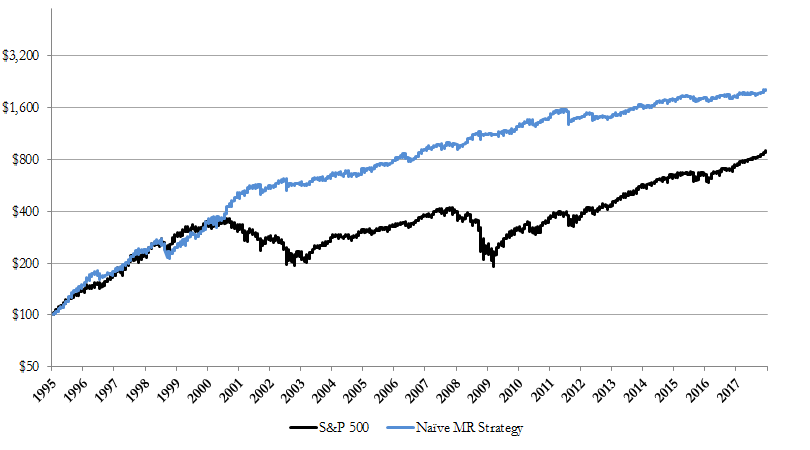
Figure 2: S&P BH vs. Naïve MR on S&P 500 Stocks (1995-2017)
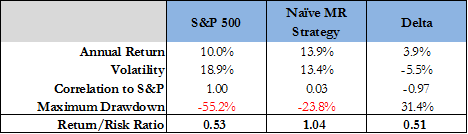
As can be easily seen in Figures 1 and 2 above, Naïve MR would have performed surprisingly well, showing significantly higher annual returns, lower volatility, and less than half the maximum drawdown (i.e. maximum peak-to-valley decline) than the S&P BH investment over the period. Additionally, Naïve MR shows a near-zero correlation to the S&P 500, indicating that it would likely act as a tremendous diversification tool in most investor portfolios. Lastly, it is apparent in Figure 1 that the naïve strategy would have been a much smoother ride than S&P BH, particularly through the prolonged bear markets associated with the Dotcom bubble and the Global Financial Crisis. (Note: This historical analysis does not account for individual tax implications, which can, as with any active strategy, affect after-tax returns.)
In order to take an even closer look at the performance profile of this type of mean reversion strategy, some additional statistical measures are provided in Figure 3 below.
Figure 3: Naïve MR - Summary Trading Strategy Statistics (1995-2017)

As presented in Figure 3, we can note a few key characteristics of the Naïve MR strategy, such as:
Moderate to High Winning Percentage: The Naïve MR strategy shows a decent percentage of winning trades of 62.3% over the analysis period, meaning that the strategy is correct in its trade direction the majority of the time. (Note: This winning percentage is actually fairly low in comparison to other more sophisticated mean reversion strategies, with many producing average win rates of 70% or more.)
Positive Average Profit Per Trade: The average profit per winner of 1.7% is slightly less than the average loss per loser of 2.2%; however, the average profit/(loss) per trade is a positive 0.20%, which is largely due to the high winning percentage of the strategy. It is important to note that although the average gain per trade is relatively small, the powerful laws of compounding returns come into effect in a big way, as there were over 31,000 trades over the full 23-year period (approx.. 1,350 trades per year). Moreover, this tremendous sample size points directly toward the robustness and statistical significance of the Naïve MR.
Low Average Market Exposure: As this strategy trades 5% positions with a maximum position count of 20, its maximum potential market exposure at any point in time was 100%. However, the average market exposure for the strategy was only 38.4% throughout the analysis period, far below its maximum potential, making it far less exposed to market shocks and prolonged downward trends. This compares to the S&P BH strategy’s perpetual 100% market exposure throughout the period.
Short Average Drawdown Length: Lastly, as a typical characteristic of many quantitative oriented strategies, the length or duration of each drawdown was relatively short, with the average drawdown length over the period being just over 72 days and the longest drawdown being 1.5 years. As a basis for comparison, the average drawdown period for the S&P BH strategy was over a year (~374 days), with the longest drawdown lasting over 4.5 years. In other words, buy and hold investors would have had to wait 4.5 years to make new equity highs in their accounts, while the Naïve MR trading strategy would have bounced back to new highs in 1.5 years.
Conclusion
After considering all the points above, we feel that many investor portfolios can benefit materially through the conservative addition of alternative, lowly-correlated strategies such as short-term mean reversion. Furthermore, as short-term mean reversion strategies typically maintain minimal average market exposure over time and consistently exhibit low or even negative correlations to traditional asset classes, they can be great alpha overlay candidates for traditional and alternative portfolios, enhancing expected returns while meaningfully augmenting portfolio diversification at the same time. Lastly, as we commonly point out at the end of our basic strategy examples, the Naïve MR strategy illustrated above is a relatively simple illustration, and there are many more high-quality, low-correlation strategies and sources of return that can be incorporated into investor portfolios to improve expected results even further.
Disclaimer: These materials have been prepared solely for informational purposes and do not constitute a recommendation to make or dispose of any investment or engage in any particular investment strategy. These materials include general information and have not been tailored for any specific recipient or recipients. Information or data shown or used in these materials were obtained from sources believed to be reliable, but accuracy is not guaranteed. Furthermore, past results are not necessarily indicative of future results. The analyses presented are based on simulated or hypothetical performance that has certain inherent limitations. Simulated or hypothetical trading programs in general are also subject to the fact that they are designed with the benefit of hindsight.