

At RQA, we often ask ourselves and our clients, “What are you truly looking for in an investment portfolio?” This is a common question put to many investors individual and institutional alike by their financial advisers, chief investment officers (CIOs), portfolio managers, and other investment professionals.
At the most basic level, we’ve found that nearly every investor is looking for a portfolio that will allow them to achieve a target level of wealth or income while assuming the least amount of risk possible. For instance, if we could all find a savings account that paid 20% in risk-free interest, we’d be happy to ditch everything else in our portfolio! So, given this desire to find a truly efficient investment framework that maximizes returns per unit of risk, how are most portfolios actually constructed in practice?
In our experience, the majority of portfolios tend to adhere to a static, buy & hold, and rebalance approach centered around a mix of global asset classes – primarily stocks and bonds, along with maybe some real estate, precious metals, and commodities for incremental diversification. The goal of these static portfolios is to provide a return profile that satisfies the investor’s needs while remaining within the guardrails of a tolerable range of estimated risk. It’s important to note, however, that in most cases the expected risk and return profiles for these portfolios are largely estimated up front using long-term historical averages as their guide. But this raises some important questions, such as:
1. Is it safe to assume these static portfolios, which are based largely on heuristics derived from long-term history, will have similar risk and return profiles in the future? And,
2. If that’s fairly uncertain (which we think it is), are there better methods of portfolio construction and rebalancing that should be considered?
Some of the Problems within Static Portfolios
First and foremost, static investment portfolios have a tendency to become unstable over time. As risks, volatilities, and correlations across markets evolve, portfolio risk and return profiles can stray far from what investors originally planned for or desired – and this can actually last for years at a time. Figure 1 below illustrates this dynamic with historical annual volatility from a static 60/40 stock and bond portfolio – using 60% in the S&P 500 Index (“Stocks” or “S&P”) and 40% in the U.S. Aggregate Bond Index (“Bonds” or “AGG”) - over the past 25 years.
Figure 1 – Rolling Annual Volatility of a Static 60/40 Portfolio
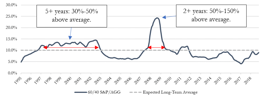
What is evident in Figure 1 above is that even though the average volatility (i.e. long-term risk estimate) for the portfolio is approximately 10%, the amount of time actually spent realizing that level of volatility is quite minimal – as the portfolio experienced long periods (years or even decades) ranging from 50% below to 150% above the long-term estimate.
To drive this point home even further, let’s say an investor is comfortable with an average risk profile that assumes 10% portfolio volatility +/- 2% (i.e. an 8%-12% range). Given the dynamics of the static 60/40 illustrated above, however, the investor would have remained within this target range only 35% of the time - meaning nearly two thirds of the time would have been spent in a sub-optimal (and often far riskier) portfolio than the investor was expecting.
An analogy here would be sitting in a sauna for half the day and then spending the rest of the day in an ice bath. On average, your body temperature would be normal, but the reality is you are likely far from comfortable throughout the day.
So, what are the consequences of this persistent inaccuracy in risk estimation? What we have found is that failure to adapt and balance a portfolio for changing conditions often leads to portfolio instability and the tendency for much larger portfolio drawdowns than is necessary.
We should note that “drawdowns” are peak-to-valley declines in portfolio value over the investment period, and are really the risks that we are concerned with most, especially as they are generally what lead investors to make undesired behavioral decisions - like panic selling to protect against further losses.
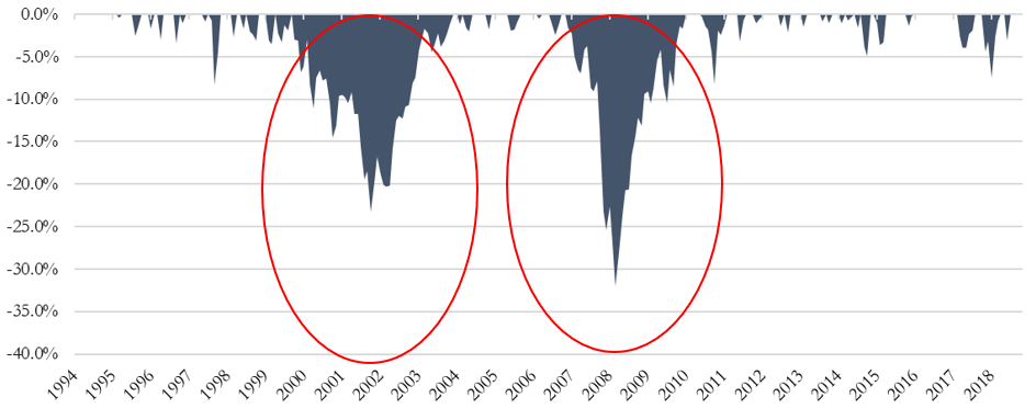
To put some further context behind all of this, we can take a look at the historical equity curve and drawdown profile of the static 60/40 Stock and Bond portfolio (with monthly rebalancing) over the past 25 years in Figures 2 and 3 below. What we see is that the static 60/40 portfolio would have performed relatively well during economic growth periods (1995-2000 and 2009-2019), but became highly unstable in environments characterized by recession and prolonged market stress (2000-2003 and 2007-2009) – particularly in the period of the global financial crisis where it would have the lost around 32% of its value and taken 5 years to get back to break even.
Figure 2 – Static 60/40 Portfolio Equity Curve (1995-2019)

Figure 3 – Static 60/40 Portfolio Drawdown Profile (1995-2019)
Using Shorter-Term Estimates Can Help
Although surprising to some, there are relatively simple, yet intelligent ways of creating and maintaining better balance and stability in portfolios over time. For starters, if we choose to dynamically adapt our portfolio allocations based on more recent market behavior (as opposed to anchoring to static, longer-term averages), we can realize material improvements in diversification and portfolio stability throughout the investment period.
To illustrate the effectiveness of using recent windows of volatility versus those that are longer-term, we can compare the accuracy of each in estimating future market volatility over the near-to-intermediate term. More specifically, we can use the market volatility of the past 60 trading days (approximately one calendar quarter) as our simple estimate or forecast for what the next month’s volatility is likely to be. We can then compare the difference between our estimates and what was actually experienced in real-time market conditions to assess our accuracy. And, we can conduct the same comparison exercise using the long-term static estimates, as well. These measures of accuracy in terms of realized volatility compared our estimates for static and dynamic for both the S&P and the AGG are presented in Figure 4 (a-b) below.
Figure 4 (a-b): Rolling Excess Volatility Over Estimate: Static Long-Term vs. Dynamic Short-Term
Figure 4-a: S&P 500 Index (Average Annual Excess Volatility Over Estimate)
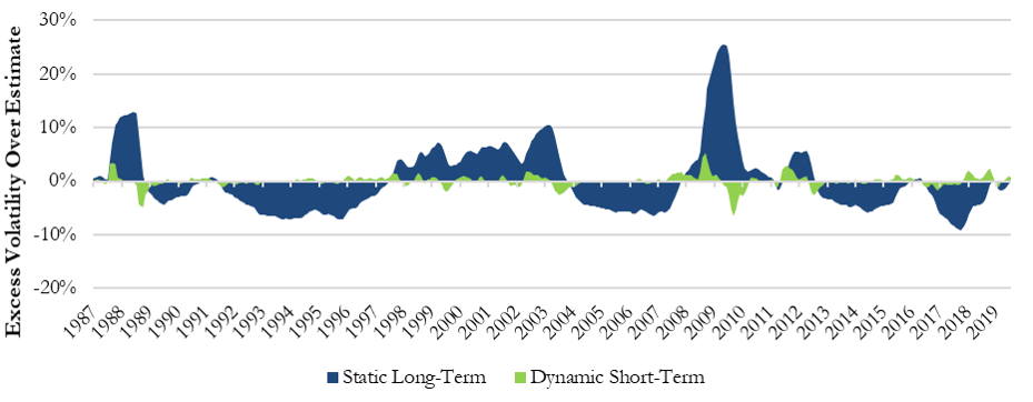
Figure 4-b: U.S. Aggregate Bond Index (Average Annual Excess Volatility Over Estimate)

As illustrated above, it is clear that using static, long-term historical averages of volatility to estimate future market behavior is poor at best, as it not only tends to deviate materially from what transpires in real-time, but it often deviates for years or even decades at a time. Meanwhile the estimates derived from the shorter-term averages provide a much more up-to-date and accurate forecast for what to expect over the coming weeks and months.
To take this one step further, we should consider these same accuracy measures (long-term vs. short-term) for estimating the expected correlation between markets, as well. Particularly as our example portfolio uses Stocks and Bonds as its core building blocks, we will want to know how these two asset classes move together over time.
Essentially, correlation is the measure of how markets behave around one another – i.e. if one goes up, what is the other likely to do? Knowing this relationship with some degree of accuracy can be extremely important, as it allows any portfolio manager to more effectively establish balance and diversification across the portfolio by pairing markets that “zig” against others that “zag”.
Just like our analysis of volatility forecasting in Figure 4 above, we have provided a similar analysis for forecasting the near-term correlation dynamics between Stocks and Bonds in Figure 5 below.
Figure 5: Rolling Correlation Estimate: Static Long-Term vs. Dynamic Short-Term for S&P/AGG

Once again, we can see that more dynamic, shorter-term estimates tend to provide a much more accurate reading over time. By using these more accurate and dynamically updated estimates of volatility and correlation for each market, we can then more accurately balance our portfolio’s risk exposures, and therefore, improve stability and insulation against market shocks and regime shifts.
Using More Accurate Estimates to Dynamically Guide Portfolios Over Time
So, how do we go about creating this more intelligently diversified and stable portfolio? First of all, we need to recognize that portfolio balance is achieved by seeking to balance risk exposures and not balancing capital allocations. This means that markets that are more erratic or volatile (i.e. higher risk) should receive relatively smaller capital allocations than those that are calmer and less volatile (i.e. lower risk). For example, most people would agree that a highly erratic investment like Bitcoin or bio-tech stocks should only be a small portion of your portfolio at most, while much less volatile and less risky assets like investment grade bonds and blue-chip stocks should command much larger allocations.
Additionally, the evolving correlations between markets should be incorporated into the analysis to make sure a high level of diversification and balance is regularly maintained – as we always want an optimal mix of assets that “zig while others zag”.
Once we have quantitatively adjusted and balanced the portfolio based on these volatility and correlation measures, we then have a more stable and efficient portfolio that can be scaled up and down in order to maintain a fairly accurate level of target volatility or portfolio risk exposure.
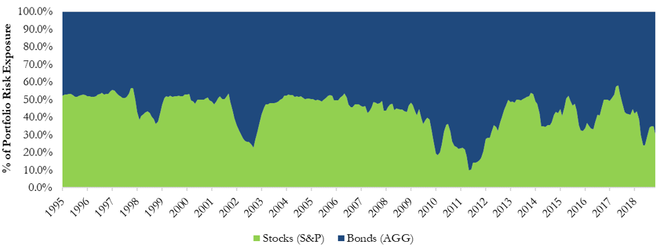
To further illustrate how this kind of dynamic approach works, we can take a look at how the portfolio allocations between Stocks and Bonds would have evolved to continually maintain balance and the desired level of portfolio risk exposure over time. As we can see in Figure 6 below, the dynamic portfolio adapts its allocations according to the changing behaviors of Stocks and Bonds (i.e. their volatilities and correlations) as we move through time. This dynamic process allows the portfolio to continually adapt and more accurately reflect real-time market conditions, and as a result, maintain more consistency in its volatility measures and risk exposures.
Figure 6 (a-b): Capital & Risk Allocations Between Stocks & Bonds Using Dynamic Adjustments
Figure 6-a: Portfolio Capital Allocations Between Stocks and Bonds

Figure 6-b: % of Average Annual Portfolio Risk Contributed by Stocks and Bonds
If we ran a similar analysis for the static 60/40 portfolio discussed above, however, we would observe that the Stocks completely dominate the portfolio from the perspective of risk exposure, as depicted in Figure 7 below, despite having a seemingly balanced capital allocation.
Figure 7 (a-b): Capital & Risk Allocations Between Stocks & Bonds Using A Static Policy
Figure 7-a: Portfolio Capital Allocations Between Stocks and Bonds

Figure 7-b: % of Average Annual Portfolio Risk Contributed by Stocks and Bonds

So how does this all play out in the end? Given the higher degree of accuracy from dynamically updating our portfolio allocations, do we actually achieve better consistency and ultimately better risk-adjusted returns over time? To better observe the portfolio level results from these different allocation methods, we can first analyze the static vs. dynamic portfolios from a risk consistency and accuracy standpoint in Figure 8 below. What we can see is that dynamic balancing and risk-level targeting techniques can produce much more consistent results with more portfolio stability over the full investment period as compared to a more static portfolio allocation policy.
Figure 8 – Average Annual Volatility of a Dynamic Stock/Bond Portfolio vs. Static 60/40

The regular maintenance of the portfolio’s diversification, balance, and volatility creates better resilience against market shocks, regime changes, and prolonged portfolio drawdowns. And as an added bonus, we can often see material improvements in expected portfolio returns as a result of these more adaptive techniques.
To drive this point home a bit further, Figures 9 - 11 below present the enhanced results these more dynamic methods can provide, particularly when scaled to target the average long-term volatility of the static 60/40 portfolio of Stocks and Bonds of approximately 10%. (Note: Results reflect dynamic use of leverage at a 3% annual interest margin rate to reach the 10% volatility target.)
Figure 9 – Dynamic S&P/AGG vs. Static 60/40 S&P/AGG Equity Curves (1995-2019)
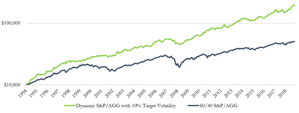
Figure 10 – Dynamic S&P/AGG vs. Static 60/40 S&P/AGG Drawdown Profile (1995-2019)

Figure 11 – Summary Performance Metrics (1995-2019)

*Note: It’s important to note that this historical analysis does not account for individual tax implications, which can, as with any active strategy, affect after-tax returns.
Conclusions and Where We Go from Here
So, what are investors both individual and institutional alike truly looking for in an investment portfolio? After operating within in the financial industry for many years, whether in investment management, investment banking, private equity, or equity research, we continue to land on the same answer to this question: At the end of the day, no one cares if their portfolio construction is 60% stocks and 40% bonds, global market cap weighted, value vs. growth focused, or any other type of typical structure. They just want a risk and return profile that optimally meets their goals, whether that’s to maximize wealth, meet or exceed scheduled pension liabilities, or generate a comfortable level of retirement income.
Yet, what we continue to find across much of the investment management industry is the widespread use of static allocation policies and portfolios based on long-term historical averages, without much consideration for meaningful dynamic adjustments as markets evolve. As we illustrated above, these static policy portfolios often completely miss their mark as markets and economic regimes change, leaving many investors in portfolios that are regularly sub-optimal, unbalanced, potentially unstable, and overall a poor fit for what the investors really need over time.
What we have found at RQA to be a major first step in addressing many of these problems is to adopt more dynamic, data-driven methods for more intelligent rebalancing and overall improvements to portfolio risk management, even if it’s just as a partial component. And as illustrated above, there are some fairly simple ways to make great strides and enhancements for basic and traditional portfolios, even by just by using more recent market behavior as your guide. That being said, we continue to discover, develop, and deploy a growing collection of new and exciting methods (especially within the field of machine learning) that we’re finding can take these potential portfolio improvements and optimizations even further.
To receive RQA Research and Updates, sign up with your email.